UQ Challenge Problem · NACA 2412 with a simple flap
Multi-Fidelity Sparse Polynomial Chaos Surrogate Models Applied to the UQ Challenge Problem
Monte Carlo-quality uncertainty assessments for a fraction of the XFOIL runs
Ashwin Sundararajan · Markus P. Rumpfkeil
University of Dayton, Ohio · AIAA SciTech 2024 Forum, Paper 2024-0708
The problem
Does the airfoil stay inside its design window?
FLAP FROM 0.7c
c/4 · MOMENT REFERENCE
HINGE · MID-THICKNESS
The use case is a sailplane delivering a payload at cruise, where the attitude must vary by less than 0.4°. That requirement is recast as a window on lift and pitching moment at a nominal 0° angle of attack. The question: how likely is the airfoil to land inside it?
Lift coefficient · Cl
0.155 to 0.265
Moment coefficient · Cm
−0.050 to −0.044
Analysis tool
XFOIL with 256 panels
Sundararajan & Rumpfkeil · University of Dayton
02 / 19
Background
Two kinds of uncertainty, two kinds of answer
Type A · irreducible
Aleatory
Inherent randomness. Collecting more data will not remove it.
Modeled as
A probability distribution, here N(μ, σ)
The answer is
A CDF and a probability of success
Type B · reducible
Epistemic
Lack of knowledge about the right value. Better information would narrow it.
Modeled as
An interval [a, b] with no assumed distribution
The answer is
Bounds on the output: its minimum and maximum
Regulators and design teams are increasingly asked to quantify epistemic uncertainty separately from aleatory uncertainty.
Sundararajan & Rumpfkeil · University of Dayton
03 / 19
The inputs
Five uncertain inputs, each with two descriptions
Parameter
Why it is uncertain
Aleatory N(μ, σ)
Epistemic [a, b]
Angle of attack
Gusts, aeroelastic twist, pitch vs. flow direction
N(0°, 0.1°)
[−0.3°, 0.3°]
Reynolds number
Exact flight speed not known
N(500000, 2500)
[492500, 507500]
Upper transition trip
Deformation, surface ripples, contamination
N(0.3c, 0.015c)
[0.255c, 0.345c]
Lower transition trip
Same causes, on the lower surface
N(0.7c, 0.021c)
[0.637c, 0.763c]
Flap deflection
Aerodynamic loads or settings
N(0°, 0.08°)
[−0.24°, 0.24°]
Epistemic intervals are ±3σ, so the aleatory and epistemic results can be compared directly.
Low Mach number assumed: compressibility is not a leading-order effect, but the exact speed, and so Re, is uncertain.
Sundararajan & Rumpfkeil · University of Dayton · c = chord length
04 / 19
The cases
Four challenge problems solved in this work
01
Baseline aleatory
All five inputs follow their normal distributions.
Result
CDFs of Cl and Cm, probability of success
02
Baseline epistemic
All five inputs can take any value in their intervals.
Result
Minimum and maximum of Cl and Cm
03
Discretization error
Repeat case 1 with most runs limited to 100 panels instead of 256.
Result
CDFs that account for mesh error
04
Uniform distribution
Repeat case 1 with uniform inputs over the epistemic intervals.
Result
CDFs and probability of success
Sundararajan & Rumpfkeil · University of Dayton
05 / 19
Method · why surrogates
Monte Carlo is the benchmark, and it is expensive
Three phases of UQ
1 · Characterize the inputs
PDFs, CDFs or bounds from data and physics
2 · Propagate them through the model
The costly step: every sample is a solver run
3 · Characterize the outputs
Statistics, CDFs or bounds of Cl and Cm
50,000
XFOIL runs for one Monte Carlo analysis
Epistemic bounds need two optimizations:
The fix: fit a cheap surrogate model to a few XFOIL runs, then run the Monte Carlo on the surrogate. This is called inexpensive Monte Carlo.
Sundararajan & Rumpfkeil · University of Dayton
06 / 19
Method · the surrogate
A polynomial chaos expansion stands in for XFOIL
Fit it once to a few XFOIL runs, then evaluate it 50,000 times at almost no cost.
Basis Ψk
Products of 1-D orthogonal polynomials, one per input. Legendre polynomials here.
Coefficients βk
Least-squares fit to XFOIL results at the training points. XFOIL itself is never modified.
Number of terms
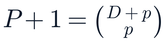
5 inputs at order 3 gives 56 terms.
Sundararajan & Rumpfkeil · University of Dayton
07 / 19
Method · multi-fidelity
Cheap runs give the trend, accurate runs correct it
α(x)
Multiplicative correction, itself a PCE
δ(x)
Additive correction, itself a PCE
LF
XFOIL with 100 panels: cheap, run often
HF
XFOIL with 256 panels: accurate, run rarely
All at once: one least-squares system
Points with HF only
These rows fit the β coefficients
Points with LF only
These rows link β, α and δ
Points with both
These rows calibrate α and δ
All P + Q + R + 3 coefficients come from one solve with singular value decomposition, instead of fitting the corrections in separate steps (Bryson and Rumpfkeil).
Sundararajan & Rumpfkeil · University of Dayton
08 / 19
Method · training points
Training points come from nested sparse grids
XFOIL runs per grid level, 5 inputs
1
11
51
151
391
903
L0
L1
L2
L3
L4
L5
Orange: grid levels used in this work (11, 51 and 151 points)
Smolyak sparse grids
Gauss-Patterson knots and a slow growth rule keep the count manageable in 5-D
Nested levels
Each level contains the one below, so earlier XFOIL runs are reused
Two fidelities
The LF grid is at least one level finer, and the HF points are a subset of it
A floor on size
Levels 0 and 1 are too small for more than a constant regular PCE in 5-D
Sundararajan & Rumpfkeil · University of Dayton · Bars to scale
09 / 19
Method · compressed sensing
Compressed sensing finds the few terms that matter
56
unknown terms at order 3 with 5 inputs
11
XFOIL runs at grid level 1
More unknowns than data, so ordinary least squares cannot pin down the model. But if only a few coefficients really matter, an L1 penalty can find them.
With 11 runs a regular PCE returns only a constant. The sparse PCE (SPCE) gives very good results.
Solver
LASSO via least angle regression (mlpack)
Choosing λ
Lowest RMSE or leave-one-out error over a sweep
Trade-off
Too large loses accuracy; too small over-fits
Used here
λ = 10⁻⁶, the most accurate in tests
Sundararajan & Rumpfkeil · University of Dayton
10 / 19
Method · test setup
How the methods were compared
50,000
Latin hypercube samples for the aleatory cases, generated once and reused for every model
±3σ
Surrogate domain in every input: over 99% of Gaussian samples and all uniform samples fall inside it
256 / 100
XFOIL panels for high-fidelity (HF) and low-fidelity (LF) runs
5,000
Function calls for the epistemic bounds: genetic algorithm (pyPI), population 100, 50 generations
Sundararajan & Rumpfkeil · University of Dayton
11 / 19
Result 1 · baseline aleatory
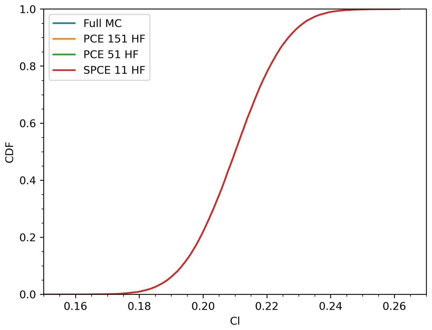
All surrogates reproduce the Monte Carlo CDFs
The four curves overlap, at very different costs
Full Monte Carlo
50,000 runs
PCE, grid level 3
151 runs
PCE, grid level 2
51 runs
Sparse PCE, grid level 1
11 runs
A regular PCE with 11 runs only returns a constant. The sparse PCE (order 3, λ = 10⁻⁶) recovers the whole curve. The Cm CDF and the tails agree as well.
Fig. 1 · CDF of Cl, Gaussian inputs
Sundararajan & Rumpfkeil · University of Dayton
12 / 19
Cost
Same answer, up to 4,545× fewer XFOIL runs
Full Monte Carlo
50,000
reference
PCE, 151 HF runs
151
331×
PCE, 51 HF runs
51
980×
Sparse PCE, 11 HF runs
11
4,545×
Each surrogate matches the Monte Carlo CDFs in the baseline aleatory case. Right column: how many times fewer XFOIL runs than the reference.
Bars to scale; bars under 2 px are drawn at 2 px
13 / 19
Result 2 · baseline epistemic
Surrogate bounds agree with XFOIL to a few digits
Model
Cl min
Cl max
Cm min
Cm max
XFOIL, 22,500 calls
0.15284
0.26594
−0.050792
−0.043478
XFOIL, 5,000 calls
0.15424
0.26504
−0.050729
−0.043527
PCE, 151 HF runs
0.15431
0.26322
−0.050733
−0.043653
PCE, 51 HF runs
0.15598
0.26479
−0.050721
−0.043658
How the bounds were found
A genetic algorithm (pyPI) searched the input intervals with population 100 for 50 generations: 5,000 calls to XFOIL or to a surrogate. A 150 × 150 search with XFOIL, 22,500 calls, checks the bounds.
Read against the requirement
The worst-case bounds fall just outside both windows: Cl 0.153 to 0.266 vs. 0.155 to 0.265, and Cm −0.0508 to −0.0435 vs. −0.050 to −0.044. With interval inputs, success is not guaranteed.
Sundararajan & Rumpfkeil · Bold digits agree with the XFOIL result
14 / 19
Result 3 · discretization error
Eleven accurate runs correct the cheap model
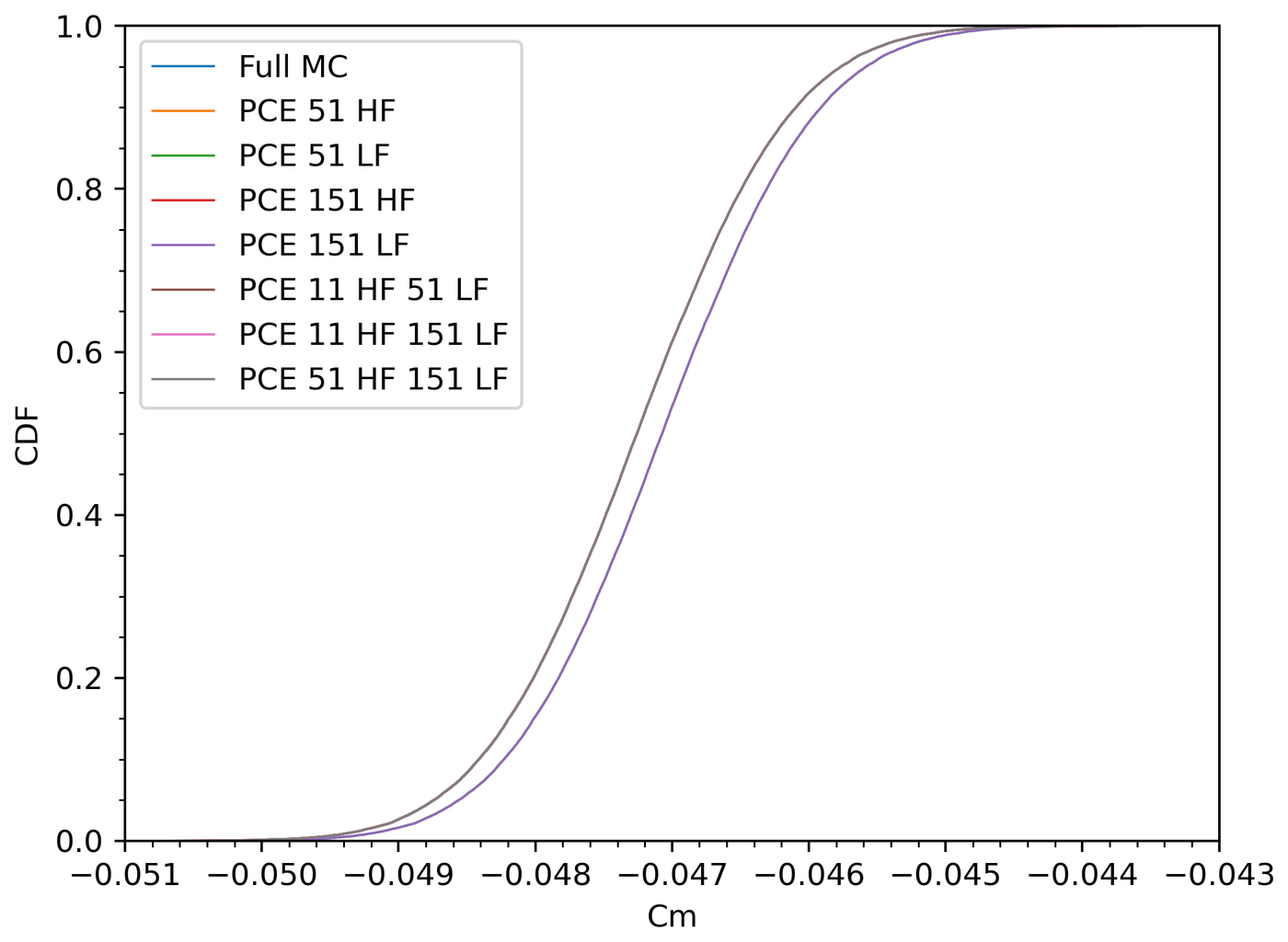
Low-fidelity runs alone shift the answer
With runs limited to 100 panels, the Cm CDF moves away from full Monte Carlo. The gap combines model error and discretization error.
A few high-fidelity runs pull it back
Adding only 11 HF runs to 51 LF runs puts the multi-fidelity PCE back on the full Monte Carlo curve, at a fraction of the cost.
Fig. 4 · CDF of Cm, two fidelity levels, Gaussian inputs
Sundararajan & Rumpfkeil · University of Dayton
15 / 19
Result 4 · uniform inputs
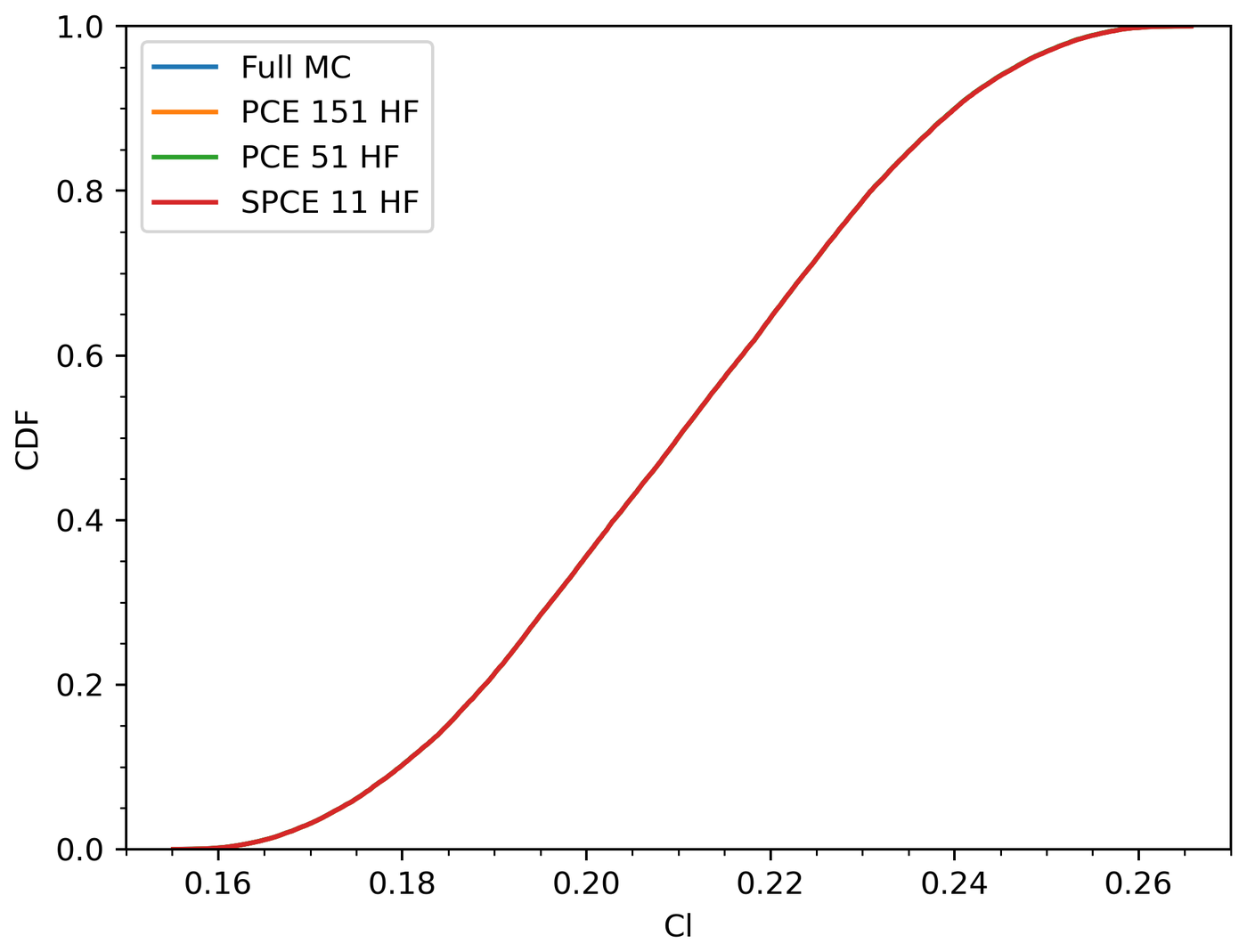
Uniform inputs: a wider spread, the same agreement
Same range, different assumption
Each input is uniform over its ±3σ interval, the same range as the epistemic case. The outputs spread more widely than with Gaussian inputs.
The surrogates still hold
Full Monte Carlo, PCE with 151 or 51 HF runs and the sparse PCE with 11 runs give the same CDFs. The sparse PCE again uses order 3 and λ = 10⁻⁶.
Fig. 5 · CDF of Cl, uniform inputs
Sundararajan & Rumpfkeil · University of Dayton
16 / 19
The answer
Probability of meeting both requirements
99.84%
with Gaussian inputs
97.68%
with uniform inputs
Full Monte Carlo, 50,000 samples
The surrogates give the same probability
Model
Gaussian
Uniform
MC, 50,000 HF runs
0.99844
0.97678
PCE, 151 HF runs
0.99846
0.97660
PCE, 51 HF runs
0.99840
0.97606
Probability that Cl is in [0.155, 0.265] and Cm is in [−0.050, −0.044] at the same time, from the same 50,000 Latin hypercube samples. Bold digits agree with full Monte Carlo.
Sundararajan & Rumpfkeil · University of Dayton
17 / 19
Conclusions
Cheap data, a few accurate runs, and sparsity
When high-fidelity runs are the dominant cost, enhance the surrogate with lower-fidelity data and compressed sensing, then run Monte Carlo on the surrogate.
Monte Carlo accuracy at a fraction of the cost
Multi-fidelity sparse PCEs match 50,000-run Monte Carlo from 11 to 151 high-fidelity runs.
Low-fidelity data is worth using
51 cheap runs plus only 11 accurate runs captured discretization error and matched full Monte Carlo.
Compressed sensing performed best
The sparse PCE worked from 11 high-fidelity runs, where a regular PCE returns only a constant.
Sundararajan & Rumpfkeil · University of Dayton
18 / 19
Questions
Thank you
Ashwin Sundararajan · Markus P. Rumpfkeil
University of Dayton, Ohio · ashwin398@gmail.com
Paper: AIAA SciTech 2024 Forum, AIAA 2024-0708, arc.aiaa.org/doi/10.2514/6.2024-0708 Challenge problem: Cary, Schaefer, Duque, Khurana and DeCarlo, “Overview of Fluid Dynamics Uncertainty Quantification Challenge Problem and Results,” AIAA SciTech, 2024.
01 / 19
←→ keys or click the slide · F full screenTap or swipe the slide to move on